In this Jupyter notebook, I’d like to experiment with ‘Hello world’ multi-class logistic regression problem - recognition of handwritten digits. I will use MxNet and its Gluon API to build a neural network. The dataset is MNIST that contains lots handwritten digits. I am going to use different optimizers that provided by MxNet to find out how they influence model training speed and prediction accuracy.
Package import
mxnet.ndis a sub-package contains all needed functionality to work with N-dimensions arraysmxnet.autogradprovides functionality to compute gradient for learning our modelsmxnet.gluonis an imperative API to build models
import mxnet as mx
from mxnet import nd, autograd, gluon
import numpy as np
import matplotlib.pyplot as plt
Configure MxNet context.
I run models on CPU here; however, MxNet also supports GPU.
model_ctx = mx.cpu()
Parameters for experiments
picture_size_pixels- the size of one picture side (in this case 28, MNIST digits are pictures with 28x28 pixels)num_inputs- how many inputs our models will have (in this case 784, each pixel on picture will have corresponding input signal)num_outputs- how many outputs our models will have (in this case we want to know what digit on a picture, each output signal is responsible for each digit from 0 till 9, thus 10)
picture_size_pixels = 28
num_inputs = picture_size_pixels * picture_size_pixels
num_outputs = 10
Preparing dataset
Transform function
First of all, I define a transform function that will be invoked on each picture of digits from the dataset to make it “digestible” for a network. It takes two parameters:
datawhich is a digit picture that represented asmxnet.nd.arraylabelwhich is the value of what digit depicted in the picture.
The function converts data into an array that will contain float numbers between 0.0 and 1.0
def transform(data, label):
    return data.astype(np.float32)/255, label.astype(np.float32)
Loading dataset
To get the MNIST dataset with MxNet is very easy. All you need is to instantiate mxnet.gluon.data.vision.MNIST objects, that’s it. It will download and store dataset on your machine. It takes three parameters:
rootwhich is the path on your machine where dataset should be stored, by default it’s~/.mxnet/datasets/mnist, *trainwhich is flag that indicate which dataset to loadTrainingorTestingtransformis the function that will be invoke on dataset item before retrieving it from dataset.
Also, I will user mxnet.gluon.data.DataLoader class to load dataset in my python script. It takes a few parameters (that you can find in documentation), but I provide only three of them:
datasetasmxnet.gluon.data.vision.MNISTobjectbatch_sizeis integer parameter to specify how many itemsDataLoadershould provide at onceshuffleshould dataset be shuffled or not.
batch_size = 64

train_data = gluon.data.DataLoader(gluon.data.vision.MNIST(train=True, transform=transform), batch_size, shuffle=True)
test_data = gluon.data.DataLoader(gluon.data.vision.MNIST(train=False, transform=transform), batch_size, shuffle=False)
Initialize network
I define general function to instantiate a network using Gluon API here.
def create_network():
    net = gluon.nn.Sequential()
    with net.name_scope():
        net.add(gluon.nn.Dense(num_outputs))
        net.collect_params().initialize(mx.init.Normal(sigma=1.), ctx=model_ctx)
    return net
Let’s break the MxNet API. First of all, mxnet.gluon.nn.Sequential - is simple object that helps build model by pushing one layer on another. We need use name_scope method that will automatically give name of parameters for added layers; these parameters will be initialized and used to create optimizer later. mxnet.gluon.nn.Dense - is a object that represent one network layer where each node has connection with each node of layer below. It our case the only one layer that has 10 outputs; the number of inputs MxNet will automatically figure out when we start feeding the network.
To Be Trained - Model Needs Feedback
To calculate how ‘wrong’ a prediction of our model is we need to use loss function. I use the softmax cross entropy function here.
softmax_cross_entropy = gluon.loss.SoftmaxCrossEntropyLoss()
Measuring model accuracy
You can compare only when you can measure. The below evaluate_accuracy function, as its name stands, evaluates network accuracy for dataset. It iterates over data_iterator and feeds data into net. We need to be sure that data and label in the same context otherwise MxNet will throw an error. It accomplished by calling as_in_context function with model_ctx context. Also, it needs to reshape data because it is a 3D array with sizes 28x28x1. Giving -1 as first item of tuple to reshape function we are telling MxNet to figure out the number of rows in a new array. Because num_inputs = 784 (which is equal to 28*28*1) thus we get an 1D array with length 784. Then we get what digit our model guessed with nd.argmax; and update accuracy object.
def evaluate_accuracy(data_iterator, net):
    accuracy = mx.metric.Accuracy()
    for data, label in data_iterator:
        data = data.as_in_context(model_ctx).reshape((-1, num_inputs))
        label = label.as_in_context(model_ctx)
        output = net(data)
        predictions = nd.argmax(output, axis=1)
        accuracy.update(preds=predictions, labels=label)
    return accuracy.get()[1]
Preparing list of optimizers
I instantiate list of optimizers as tuples, where the first item is the name that MxNet can recognize, the second is parameters for the optimizer (I took them from Gluon tutorial part about network optimization), the third one is the color with which prediction accuracy will be depicted on plots and the last one is the labels for plots. Nice article about optimizers. I found it very interesting with right level of details.
optimizers = [
    ('sgd', {'learning_rate': 0.1}, 'red', 'sgd'),
    ('sgd', {'learning_rate': 0.2, 'momentum': 0.9 }, 'blue', 'sgd-momentum'),
    ('adagrad', {'learning_rate': 0.9}, 'green', 'adagrad'),
    ('rmsprop', {'learning_rate': 0.03, 'gamma1': 0.9}, 'orange', 'rmsprop'),
    ('adadelta', {'rho': 0.9999}, 'black', 'adadelta')
]
Experiments
Following code snippet contains code to run the networks with different optimizers. Each network will run training over 5 epochs. I am recording accuracy at each of the epoch, and then pass it to build a plot and then printing to notebook output.
I will highlight the most interesting lines of the code here:
trainer = gluon.Trainer(net.collect_params(), name, params)
This line is instantiating optimizer for the network with its parameters, optimizer’s name and optimizer’s parameters that we set earlier.
with autograd.record():
    output = net(data)
    loss = softmax_cross_entropy(output, label)
loss.backward()
trainer.step(batch_size)
Here is where all model’s training occurs. We do a backpropagation procedure; compute a direction in which our model moves in the trainings and correlate it that the model can make a better predictions next time.
epochs = 5

fig = plt.figure(figsize=(20, 9))
train_plot = fig.add_subplot(1, 2, 1)
test_plot = fig.add_subplot(1, 2, 2)

final_accuracy = {}

for optimizer in optimizers:
    name, params, color, key = optimizer

    net = create_network()
    trainer = gluon.Trainer(net.collect_params(), name, params)
    test_accuracy = []
    train_accuracy = []

    for e in range(epochs):
        for data, label in train_data:
            data = data.as_in_context(model_ctx).reshape((-1, num_inputs))
            label = label.as_in_context(model_ctx)
            with autograd.record():
                output = net(data)
                loss = softmax_cross_entropy(output, label)
            loss.backward()
            trainer.step(batch_size)

        test_accuracy.append(evaluate_accuracy(test_data, net))
        train_accuracy.append(evaluate_accuracy(train_data, net))


    y_ticks = [e + 1 for e in range(epochs)]
    x_ticks = np.arange(0.75, 1.0, 0.05)
    def create_plot(line_plot, data, kind):
        line_plot.plot(data, y_ticks, c=color, label=key)
        line_plot.legend(loc='upper left')
        line_plot.set_title("Model's {} prediction accuracy trends".format(kind))
        line_plot.set_xlabel('Accuracy')
        line_plot.set_xticks(x_ticks)
        line_plot.set_ylabel('Epochs')
        line_plot.set_yticks(y_ticks)

    create_plot(train_plot, train_accuracy, 'train')
    create_plot(test_plot, test_accuracy, 'test')

    final_accuracy[key] = (train_accuracy, test_accuracy)

plt.show()
for name, acc in final_accuracy.items():
    print('Optimizer: "{}"'.format(name))
    train, test = acc
    for i in range(epochs):
        print('Train accuracy: {:.2%}, Test accuracy: {:.2%}'.format(train[i], test[i]))
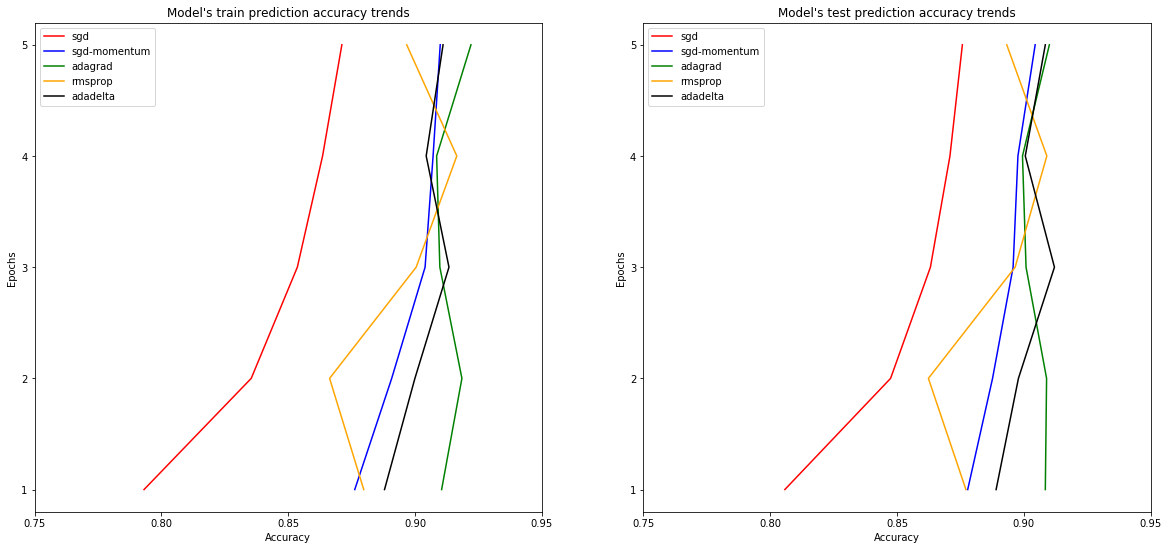
    Optimizer: "sgd"
    Train accuracy: 80.18%, Test accuracy: 81.41%
    Train accuracy: 83.99%, Test accuracy: 84.86%
    Train accuracy: 85.59%, Test accuracy: 86.08%
    Train accuracy: 86.69%, Test accuracy: 87.23%
    Train accuracy: 87.42%, Test accuracy: 87.67%
    Optimizer: "sgd-momentum"
    Train accuracy: 88.50%, Test accuracy: 88.85%
    Train accuracy: 90.59%, Test accuracy: 90.26%
    Train accuracy: 90.81%, Test accuracy: 90.53%
    Train accuracy: 90.95%, Test accuracy: 90.28%
    Train accuracy: 91.53%, Test accuracy: 90.67%
    Optimizer: "adagrad"
    Train accuracy: 90.48%, Test accuracy: 90.08%
    Train accuracy: 91.50%, Test accuracy: 90.59%
    Train accuracy: 92.29%, Test accuracy: 91.30%
    Train accuracy: 91.83%, Test accuracy: 90.58%
    Train accuracy: 92.39%, Test accuracy: 91.49%
    Optimizer: "rmsprop"
    Train accuracy: 88.99%, Test accuracy: 88.26%
    Train accuracy: 90.35%, Test accuracy: 90.28%
    Train accuracy: 90.29%, Test accuracy: 89.79%
    Train accuracy: 89.37%, Test accuracy: 88.71%
    Train accuracy: 91.70%, Test accuracy: 91.12%
    Optimizer: "adadelta"
    Train accuracy: 88.63%, Test accuracy: 88.67%
    Train accuracy: 89.66%, Test accuracy: 89.48%
    Train accuracy: 89.62%, Test accuracy: 89.60%
    Train accuracy: 91.19%, Test accuracy: 90.62%
    Train accuracy: 89.68%, Test accuracy: 89.34%
Sum up
For the task of recognizing handwritten digits all optimizers provide feedback for reasonable prediction. As you can see from plots the model with ‘sgd’ optimizer has sloping prediction rate.